Day 30: Capstone - Full Clinical Reporting Workflow

Survival · Safety · Lab · Subgroups across the pharmaverse

Back to Roadmap

1 Overview

Day 30 is the capstone. A single Quarto document drives a complete Efficacy · Safety · Lab reporting workflow using five pharmaverse packages and eight figures.

Domain	Package	Key output
Data	pharmaverseadam	ADSL, ADAE, ADLB
Efficacy	ggsurvfit + survival	KM curve · Forest plot
Safety	ggplot2	AE body system · Preferred terms
Lab	ggplot2	Lab trend · Grade distribution
Demog	gtsummary + ggplot2	Table + violin · Swimmer plot

---

2 Setup

library(ggsurvfit)
library(gtsummary)
library(survival)
library(broom)
library(purrr)
library(pharmaverseadam)
library(dplyr)
library(ggplot2)
library(stringr)
library(knitr)

# ── Load datasets ────────────────────────────────────────────────────────────
adsl <- pharmaverseadam::adsl
adae <- pharmaverseadam::adae
adlb <- pharmaverseadam::adlb

cat("adsl:", nrow(adsl), "rows |", ncol(adsl), "cols\n")

adsl: 306 rows | 54 cols

cat("adae:", nrow(adae), "rows |", ncol(adae), "cols\n")

adae: 1191 rows | 107 cols

cat("adlb:", nrow(adlb), "rows |", ncol(adlb), "cols\n")

adlb: 83652 rows | 115 cols

# Show what treatment columns adae actually carries
ae_trt_cols <- intersect(names(adae), c("TRTA", "TRTP", "TRT01A", "TRT01P", "ARM"))
cat("Treatment columns in adae:", if (length(ae_trt_cols)) ae_trt_cols else "NONE", "\n")

Treatment columns in adae: ARM TRT01P TRT01A 

# ── Subject-to-treatment lookup from ADSL ───────────────────────────────────
# pharmaverseadam::adae may not carry a treatment column at all.
# Safe pattern: distinct(USUBJID, event) first, THEN left_join treatment.
# This avoids any dependency on adae containing a treatment variable,
# and avoids .x/.y conflicts from joining a column that already exists.
trt_lookup <- adsl |>
  dplyr::filter(SAFFL == "Y") |>
  dplyr::select(USUBJID, TRT01A) |>
  dplyr::distinct()

cat("trt_lookup rows:", nrow(trt_lookup), "\n")

trt_lookup rows: 254 

cat("TRT01A levels:", paste(sort(unique(trt_lookup$TRT01A)), collapse = "; "), "\n")

TRT01A levels: Placebo; Xanomeline High Dose; Xanomeline Low Dose 

# ── Shared colour palette ────────────────────────────────────────────────────
trt_col <- c(
  "Placebo"              = "#4E79A7",
  "Xanomeline High Dose" = "#F28E2B",
  "Xanomeline Low Dose"  = "#59A14F"
)

# ── Shared ggplot2 theme ─────────────────────────────────────────────────────
theme_clin <- function(base = 11) {
  theme_minimal(base_size = base) +
    theme(
      plot.title       = element_text(face = "bold"),
      plot.subtitle    = element_text(colour = "grey40", size = base - 1),
      legend.position  = "bottom",
      panel.grid.minor = element_blank(),
      strip.text       = element_text(face = "bold")
    )
}

# ── Derive OS ADTTE from ADSL ────────────────────────────────────────────────
# adtte inherits ALL adsl columns via filter() + mutate() (not transmute()).
# CNSR = 0 (death = event) | 1 (censored)  [ADaM convention]
adtte <- adsl |>
  dplyr::filter(SAFFL == "Y") |>
  dplyr::mutate(
    TRTP = TRT01P,
    CNSR = dplyr::if_else(!is.na(DTHDT), 0L, 1L),
    AVAL = dplyr::case_when(
      !is.na(DTHDT)    ~ as.numeric(DTHDT    - TRTSDT),
      !is.na(LSTALVDT) ~ as.numeric(LSTALVDT - TRTSDT),
      !is.na(EOSDT)    ~ as.numeric(EOSDT    - TRTSDT),
      !is.na(TRTEDT)   ~ as.numeric(TRTEDT   - TRTSDT) + 1,
      TRUE             ~ NA_real_
    )
  ) |>
  dplyr::filter(!is.na(AVAL), AVAL >= 0)

cat("\nDerived ADTTE:", nrow(adtte), "rows |",
    "Events:", sum(adtte$CNSR == 0), "|",
    "Censored:", sum(adtte$CNSR == 1), "\n")

Derived ADTTE: 252 rows | Events: 3 | Censored: 249 

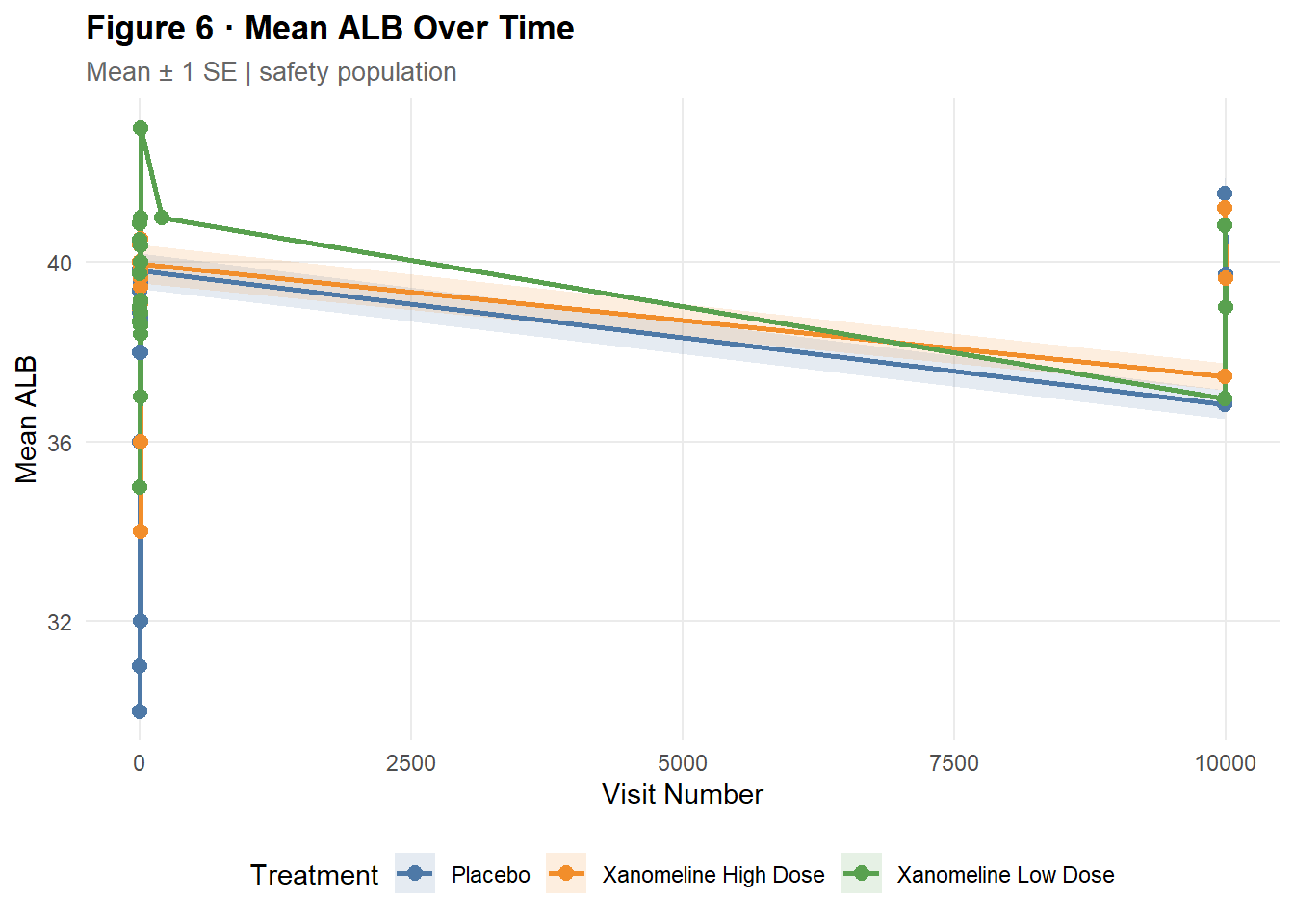
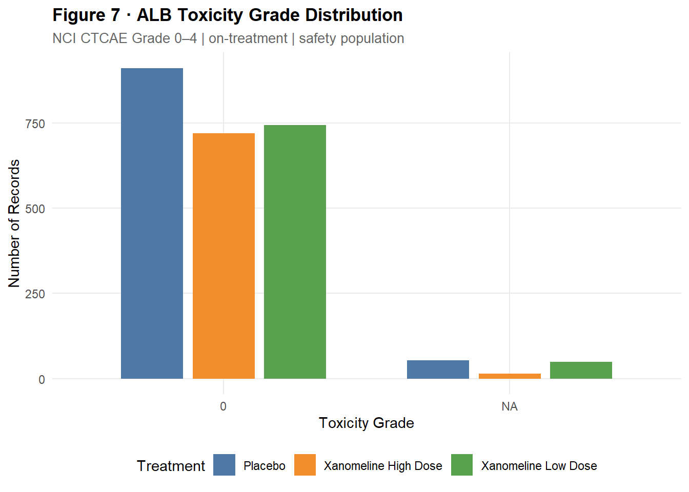
# ── Safety-population N per arm (denominator for AE %) ──────────────────────
trt_n <- adsl |>
  dplyr::filter(SAFFL == "Y") |>
  dplyr::count(TRT01A, name = "N_TRT")

# ── First available lab PARAMCD ──────────────────────────────────────────────
lab_param <- unique(adlb$PARAMCD)[1]
cat("\nLab parameter for Figures 6 & 7:", lab_param, "\n")

Lab parameter for Figures 6 & 7: ALB 

---

3 Efficacy

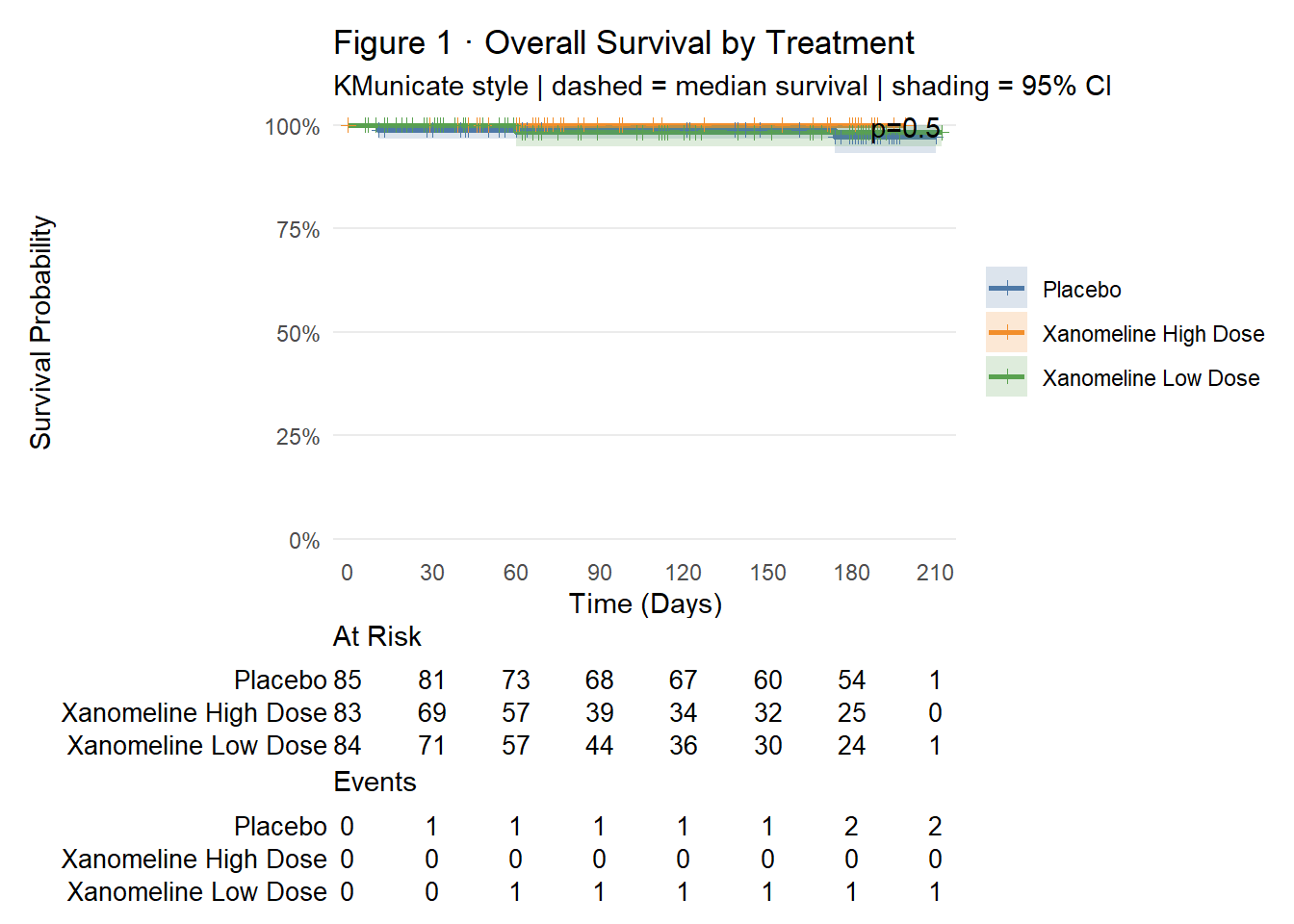
3.1 Figure 1 · Overall Survival - KM Curve

# survfit2() is required for add_pvalue().
# Layering order: geoms → scales → theme → add_risktable() last.

km_fit <- survfit2(Surv_CNSR(AVAL, CNSR) ~ TRTP, data = adtte)
km_fit

Call: survfit(formula = Surv_CNSR(AVAL, CNSR) ~ TRTP, data = adtte)

                           n events median 0.95LCL 0.95UCL
TRTP=Placebo              85      2     NA      NA      NA
TRTP=Xanomeline High Dose 83      0     NA      NA      NA
TRTP=Xanomeline Low Dose  84      1     NA      NA      NA

km_fit |>
  ggsurvfit(linewidth = 1) +
  add_confidence_interval() +
  add_censor_mark(shape = 3, size = 1.5) +
  add_quantile(y_value = 0.5, color = "grey40",
               linewidth = 0.75, linetype = "dashed") +
  add_pvalue(location = "annotation", prepend_p = TRUE) +
  scale_ggsurvfit() +
  scale_colour_manual(values = trt_col) +
  scale_fill_manual(values = trt_col) +
  theme_ggsurvfit_KMunicate() +
  labs(
    title    = "Figure 1 \u00b7 Overall Survival by Treatment",
    subtitle = "KMunicate style | dashed = median survival | shading = 95% CI",
    x        = "Time (Days)",
    y        = "Survival Probability"
  ) +
  add_risktable(
    risktable_stats = c("n.risk", "cum.event"),
    stats_label     = list(n.risk = "At Risk", cum.event = "Events")
  )

---

3.2 Figure 2 · Subgroup Forest Plot

# Subgroup levels are detected dynamically from adtte.
# tryCatch() silently skips subgroups where coxph fails.

subgroup_spec <- list(
  list(var = "AGEGR1", label = "Age Group"),
  list(var = "SEX",    label = "Sex"),
  list(var = "RACE",   label = "Race")
)

fit_subgroup_cox <- function(df, var_label, level_val) {
  tryCatch({
    fit <- survival::coxph(Surv_CNSR(AVAL, CNSR) ~ TRTP, data = df)
    broom::tidy(fit, exponentiate = TRUE, conf.int = TRUE) |>
      dplyr::slice(1) |>
      dplyr::mutate(
        var_label = var_label,
        level     = as.character(level_val),
        panel_lbl = paste0(var_label, ": ", level_val)
      )
  }, error = function(e) dplyr::tibble())
}

forest_df <- purrr::map_dfr(subgroup_spec, function(sg) {
  purrr::map_dfr(unique(adtte[[sg$var]]), function(lv) {
    fit_subgroup_cox(adtte[adtte[[sg$var]] == lv, ], sg$label, lv)
  })
}) |>
  dplyr::filter(!is.na(estimate), !is.na(conf.low), !is.na(conf.high))

cat("Forest plot rows:", nrow(forest_df), "\n")

Forest plot rows: 4 

ggplot(forest_df,
       aes(x = estimate, y = reorder(panel_lbl, estimate),
           xmin = conf.low, xmax = conf.high, colour = var_label)) +
  geom_point(size = 3.5) +
  geom_errorbarh(height = 0.35, linewidth = 0.8) +
  geom_vline(xintercept = 1, linetype = "dashed",
             colour = "red", linewidth = 0.7) +
  scale_x_log10() +
  labs(
    title    = "Figure 2 \u00b7 Subgroup Forest Plot (Hazard Ratios)",
    subtitle = "Cox PH per subgroup | log scale | reference = Placebo",
    x        = "Hazard Ratio (log scale)",
    y        = NULL,
    colour   = "Subgroup"
  ) +
  theme_clin()

---

4 Demographics

4.1 Table 1 · Baseline Characteristics

# adtte inherits all adsl columns -- no join needed.
adtte |>
  dplyr::select(AGE, AGEGR1, SEX, RACE, TRTP) |>
  gtsummary::tbl_summary(
    by        = TRTP,
    label     = list(AGE    ~ "Age (years)", AGEGR1 ~ "Age Group",
                     SEX    ~ "Sex",         RACE   ~ "Race"),
    statistic = list(
      all_continuous()  ~ "{mean} ({sd})",
      all_categorical() ~ "{n} ({p}%)"
    ),
    digits  = all_continuous() ~ 1,
    missing = "no"
  ) |>
  gtsummary::add_overall() |>
  gtsummary::bold_labels() |>
  gtsummary::as_kable()

Characteristic	Overall N = 252	Placebo N = 85	Xanomeline High Dose N = 83	Xanomeline Low Dose N = 84
Age (years)	75.1 (8.3)	75.3 (8.6)	74.3 (7.9)	75.7 (8.3)
Age Group
>64	219 (87%)	71 (84%)	72 (87%)	76 (90%)
18-64	33 (13%)	14 (16%)	11 (13%)	8 (9.5%)
Sex
F	142 (56%)	52 (61%)	40 (48%)	50 (60%)
M	110 (44%)	33 (39%)	43 (52%)	34 (40%)
Race
AMERICAN INDIAN OR ALASKA NATIVE	1 (0.4%)	0 (0%)	1 (1.2%)	0 (0%)
BLACK OR AFRICAN AMERICAN	23 (9.1%)	8 (9.4%)	9 (11%)	6 (7.1%)
WHITE	228 (90%)	77 (91%)	73 (88%)	78 (93%)

---

4.2 Figure 3 · Age Distribution by Treatment

adsl |>
  dplyr::filter(SAFFL == "Y") |>
  ggplot(aes(x = TRT01A, y = AGE, fill = TRT01A)) +
  geom_violin(alpha = 0.55, trim = FALSE) +
  geom_boxplot(width = 0.12, fill = "white",
               outlier.shape = NA, linewidth = 0.6) +
  geom_jitter(width = 0.08, size = 0.9, alpha = 0.35) +
  stat_summary(fun = mean, geom = "point",
               shape = 23, size = 3.5, fill = "yellow", colour = "black") +
  scale_fill_manual(values = trt_col) +
  labs(
    title    = "Figure 3 \u00b7 Age Distribution by Treatment Arm",
    subtitle = "Violin + boxplot + jitter | \u25c6 = mean",
    x        = NULL,
    y        = "Age (years)"
  ) +
  theme_clin() +
  theme(legend.position = "none",
        axis.text.x = element_text(size = 9))

---

5 Safety - Adverse Events

5.1 Figure 4 · AE Incidence by Body System

# Key pattern: distinct(USUBJID, AEBODSYS) first -- no treatment column needed.
# Then left_join trt_lookup to add TRT01A safely, then count() and %.
# This works regardless of whether adae carries a treatment column.

ae_soc <- adae |>
  dplyr::filter(SAFFL == "Y", TRTEMFL == "Y") |>
  dplyr::distinct(USUBJID, AEBODSYS) |>
  dplyr::left_join(trt_lookup, by = "USUBJID") |>
  dplyr::count(TRT01A, AEBODSYS, name = "n_subj") |>
  dplyr::left_join(trt_n, by = "TRT01A") |>
  dplyr::mutate(pct = n_subj / N_TRT * 100)

top_soc <- ae_soc |>
  dplyr::group_by(AEBODSYS) |>
  dplyr::summarise(max_pct = max(pct), .groups = "drop") |>
  dplyr::slice_max(max_pct, n = 10) |>
  dplyr::pull(AEBODSYS)

ae_soc |>
  dplyr::filter(AEBODSYS %in% top_soc) |>
  dplyr::mutate(AEBODSYS = stringr::str_wrap(AEBODSYS, width = 38)) |>
  ggplot(aes(x = pct,
             y = reorder(AEBODSYS, pct),
             fill = TRT01A)) +
  geom_col(position = position_dodge(width = 0.75), width = 0.65) +
  scale_fill_manual(values = trt_col) +
  labs(
    title    = "Figure 4 \u00b7 TEAEs by Body System (Top 10)",
    subtitle = "% subjects with \u22651 TEAE | treatment-emergent | safety population",
    x        = "% Subjects",
    y        = NULL,
    fill     = "Treatment"
  ) +
  theme_clin()

---

5.2 Figure 5 · Top 15 Preferred Terms - Cleveland Dot Plot

# Same pattern: distinct on AE columns only, then join treatment.

top_pts <- adae |>
  dplyr::filter(SAFFL == "Y", TRTEMFL == "Y") |>
  dplyr::distinct(USUBJID, AEDECOD) |>
  dplyr::count(AEDECOD, sort = TRUE) |>
  dplyr::slice_head(n = 15) |>
  dplyr::pull(AEDECOD)

ae_pt <- adae |>
  dplyr::filter(SAFFL == "Y", TRTEMFL == "Y", AEDECOD %in% top_pts) |>
  dplyr::distinct(USUBJID, AEDECOD) |>
  dplyr::left_join(trt_lookup, by = "USUBJID") |>
  dplyr::count(TRT01A, AEDECOD, name = "n_subj") |>
  dplyr::left_join(trt_n, by = "TRT01A") |>
  dplyr::mutate(pct = n_subj / N_TRT * 100)

ggplot(ae_pt,
       aes(x = pct,
           y = reorder(AEDECOD, pct),
           colour = TRT01A)) +
  geom_line(aes(group = AEDECOD), colour = "grey80", linewidth = 0.8) +
  geom_point(size = 3.5) +
  scale_colour_manual(values = trt_col) +
  labs(
    title    = "Figure 5 \u00b7 Top 15 TEAEs by Preferred Term",
    subtitle = "% subjects with \u22651 TEAE | connected = same PT across arms",
    x        = "% Subjects",
    y        = NULL,
    colour   = "Treatment"
  ) +
  theme_clin()

---

6 Lab Safety

6.1 Figure 6 · Mean Lab Value Over Time

lab_trend <- adlb |>
  dplyr::filter(SAFFL == "Y", PARAMCD == lab_param,
                !is.na(AVAL), !is.na(AVISITN)) |>
  dplyr::group_by(TRTA, AVISIT, AVISITN) |>
  dplyr::summarise(
    mean_val = mean(AVAL, na.rm = TRUE),
    se_val   = sd(AVAL,   na.rm = TRUE) / sqrt(dplyr::n()),
    .groups  = "drop"
  )

ggplot(lab_trend,
       aes(x = AVISITN, y = mean_val, colour = TRTA, fill = TRTA)) +
  geom_ribbon(aes(ymin = mean_val - se_val, ymax = mean_val + se_val),
              alpha = 0.15, colour = NA) +
  geom_line(linewidth = 1) +
  geom_point(size = 2.5) +
  scale_colour_manual(values = trt_col) +
  scale_fill_manual(values = trt_col) +
  labs(
    title    = paste0("Figure 6 \u00b7 Mean ", lab_param, " Over Time"),
    subtitle = "Mean \u00b1 1 SE | safety population",
    x        = "Visit Number",
    y        = paste0("Mean ", lab_param),
    colour   = "Treatment",
    fill     = "Treatment"
  ) +
  theme_clin()

---

6.2 Figure 7 · Lab Toxicity Grade Distribution

# ATOXGR = on-treatment NCI CTCAE grade. Falls back to CHG/PCHG histogram.

if ("ATOXGR" %in% names(adlb)) {
  adlb |>
    dplyr::filter(SAFFL == "Y", PARAMCD == lab_param, !is.na(ATOXGR)) |>
    dplyr::count(TRTA, ATOXGR) |>
    dplyr::mutate(ATOXGR = factor(ATOXGR, levels = 0:4)) |>
    ggplot(aes(x = ATOXGR, y = n, fill = TRTA)) +
    geom_col(position = position_dodge(width = 0.75), width = 0.65) +
    scale_fill_manual(values = trt_col) +
    labs(
      title    = paste0("Figure 7 \u00b7 ", lab_param,
                        " Toxicity Grade Distribution"),
      subtitle = "NCI CTCAE Grade 0\u20134 | on-treatment | safety population",
      x        = "Toxicity Grade", y = "Number of Records", fill = "Treatment"
    ) +
    theme_clin()
} else {
  chg_col <- if ("PCHG" %in% names(adlb)) "PCHG" else "CHG"
  adlb |>
    dplyr::filter(SAFFL == "Y", PARAMCD == lab_param,
                  !is.na(.data[[chg_col]])) |>
    ggplot(aes(x = .data[[chg_col]], fill = TRTA)) +
    geom_histogram(bins = 30, alpha = 0.65, position = "identity") +
    scale_fill_manual(values = trt_col) +
    labs(
      title    = paste0("Figure 7 \u00b7 ", lab_param, " Change from Baseline"),
      subtitle = paste0(chg_col, " | safety population"),
      x = chg_col, y = "Count", fill = "Treatment"
    ) +
    theme_clin()
}

---

7 Swimmer Plot

7.1 Figure 8 · Per-Subject Treatment Duration and Death Events

swimmer <- adsl |>
  dplyr::filter(SAFFL == "Y", !is.na(TRTSDT), !is.na(TRTEDT)) |>
  dplyr::mutate(
    trt_dur = as.numeric(TRTEDT - TRTSDT),
    dth_day = as.numeric(DTHDT  - TRTSDT),
    trt_arm = dplyr::case_when(
      stringr::str_detect(TRT01A, "High") ~ "Xanomeline\nHigh Dose",
      stringr::str_detect(TRT01A, "Low")  ~ "Xanomeline\nLow Dose",
      TRUE                                ~ "Placebo"
    )
  ) |>
  dplyr::filter(trt_dur >= 0) |>
  dplyr::arrange(trt_arm, trt_dur) |>
  dplyr::mutate(subj_rank = dplyr::row_number())

ggplot(swimmer) +
  geom_segment(
    aes(x = 0, xend = trt_dur,
        y = subj_rank, yend = subj_rank,
        colour = trt_arm),
    linewidth = 1.6, alpha = 0.75
  ) +
  geom_point(
    data  = dplyr::filter(swimmer, !is.na(dth_day)),
    aes(x = dth_day, y = subj_rank),
    shape = 4, size = 2.5, stroke = 1.2, colour = "black"
  ) +
  facet_grid(trt_arm ~ ., scales = "free_y", space = "free_y") +
  scale_colour_manual(values = c(
    "Xanomeline\nHigh Dose" = "#F28E2B",
    "Xanomeline\nLow Dose"  = "#59A14F",
    "Placebo"               = "#4E79A7"
  )) +
  labs(
    title    = "Figure 8 \u00b7 Swimmer Plot \u2014 Treatment Duration & Death Events",
    subtitle = "Bars = days on treatment | \u00d7 = death | sorted by arm then duration",
    x        = "Days from Treatment Start",
    y        = "Subject (anonymised rank)",
    caption  = "\u00d7 = death event"
  ) +
  theme_clin() +
  theme(axis.text.y     = element_blank(),
        axis.ticks.y    = element_blank(),
        legend.position = "none",
        strip.text.y    = element_text(angle = 0, size = 9))

---

8 Validation

cat("\n=== Day 30 Validation ===\n\n")

=== Day 30 Validation ===

cat("Check  1 - adsl rows              :", nrow(adsl),    "\n")

Check  1 - adsl rows              : 306 

cat("Check  2 - adae rows              :", nrow(adae),    "\n")

Check  2 - adae rows              : 1191 

cat("Check  3 - adlb rows              :", nrow(adlb),    "\n")

Check  3 - adlb rows              : 83652 

cat("Check  4 - trt_lookup rows        :", nrow(trt_lookup), "\n")

Check  4 - trt_lookup rows        : 254 

cat("Check  5 - adtte rows (derived)   :", nrow(adtte),   "\n")

Check  5 - adtte rows (derived)   : 252 

cat("Check  6 - Events (CNSR=0)        :", sum(adtte$CNSR == 0), "\n")

Check  6 - Events (CNSR=0)        : 3 

cat("Check  7 - KM strata              :", length(km_fit$strata), "\n")

Check  7 - KM strata              : 3 

cat("Check  8 - Forest plot rows       :", nrow(forest_df), "\n")

Check  8 - Forest plot rows       : 4 

cat("Check  9 - AE SOC rows            :", nrow(ae_soc),  "\n")

Check  9 - AE SOC rows            : 60 

cat("Check 10 - AE PT rows             :", nrow(ae_pt),   "\n")

Check 10 - AE PT rows             : 45 

cat("Check 11 - Lab trend rows         :", nrow(lab_trend), "\n")

Check 11 - Lab trend rows         : 63 

cat("Check 12 - Swimmer rows           :", nrow(swimmer), "\n")

Check 12 - Swimmer rows           : 252 

cat("Check 13 - Log-rank p             :", format(survfit2_p(km_fit), digits = 4), "\n")

Check 13 - Log-rank p             : p=0.5 

cat("\nAll checks complete\n")

All checks complete

---

9 Key Takeaways

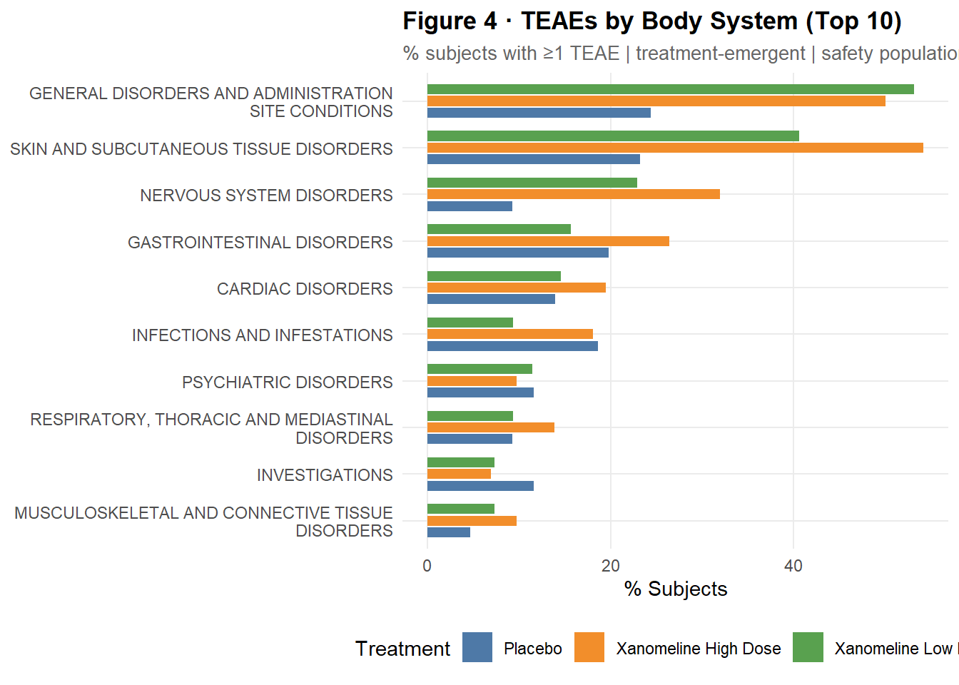
1. pharmaverseadam::adae carries no treatment column – never pre-join it into adae; instead use distinct(USUBJID, event) first, then left_join(trt_lookup, by = "USUBJID") to add TRT01A right before count()
2. Pre-joining creates .x/.y duplicates if the column already exists in adae – the safe pattern is: filter → distinct on event columns only → join → count
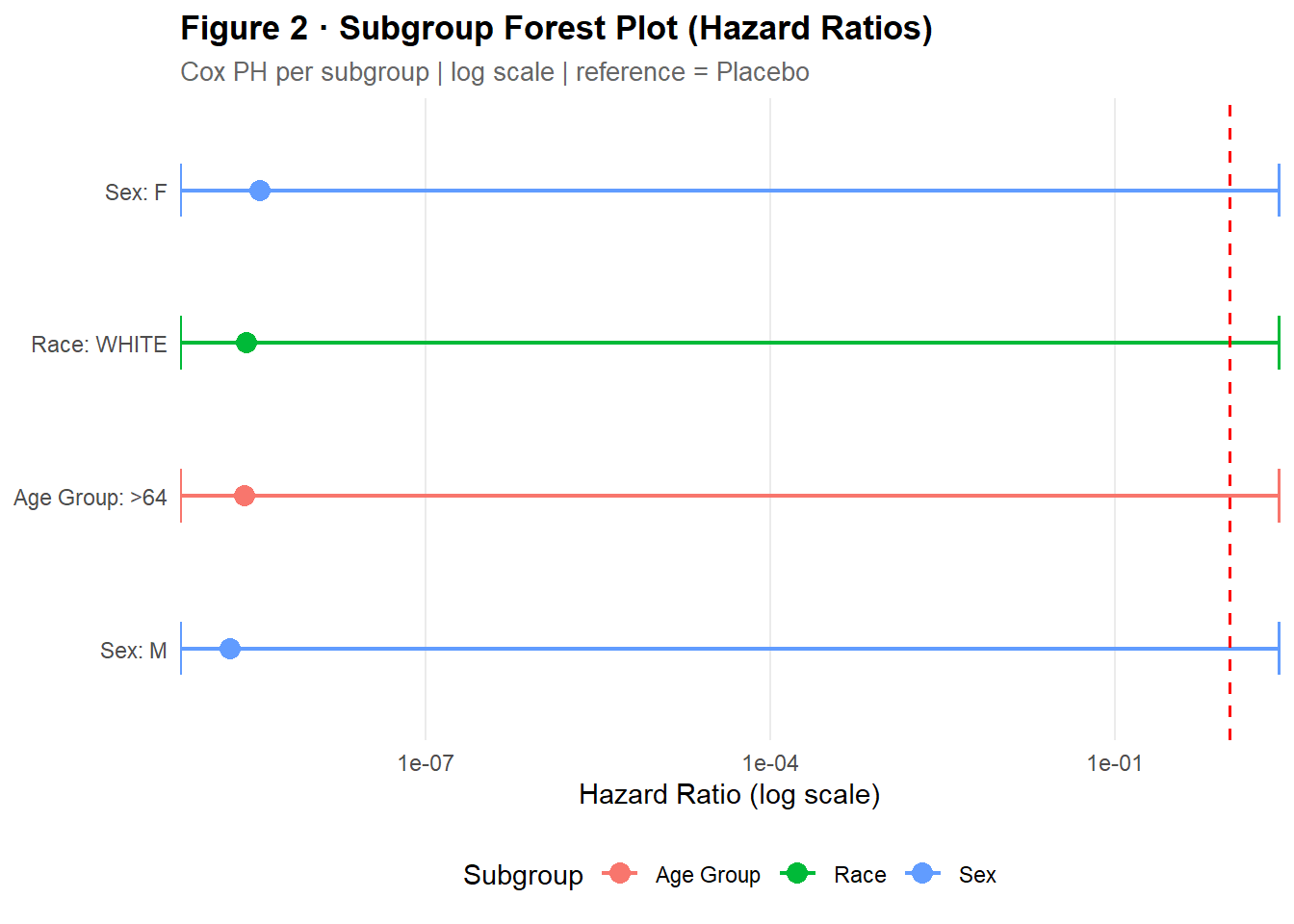
3. adtte inherits all adsl columns via filter() + mutate(), not transmute() – AGE, AGEGR1, SEX, RACE are already present; never re-join adsl into adtte
4. survfit2() + Surv_CNSR() required for add_pvalue(); Surv_CNSR() handles ADaM CNSR coding in survfit2() and coxph()
5. add_risktable() must be last in the ggsurvfit chain – it wraps the plot with patchwork and cannot be further modified
6. theme_clin() + trt_col defined once in setup, applied everywhere with scale_fill_manual(values = trt_col) and scale_colour_manual(values = trt_col)
7. Dynamic lab_param from unique(adlb$PARAMCD)[1] avoids hard-coded parameter codes – the code ports to any study without changes

---

10 Resources

• ggsurvfit: https://www.danieldsjoberg.com/ggsurvfit/
• gtsummary: https://www.danieldsjoberg.com/gtsummary/
• pharmaverse: https://pharmaverse.org
• CDISC ADaM IG: https://www.cdisc.org/standards/foundational/adam

---

End of Day 30 - 30 Days of Pharmaverse complete.

---